Introduction
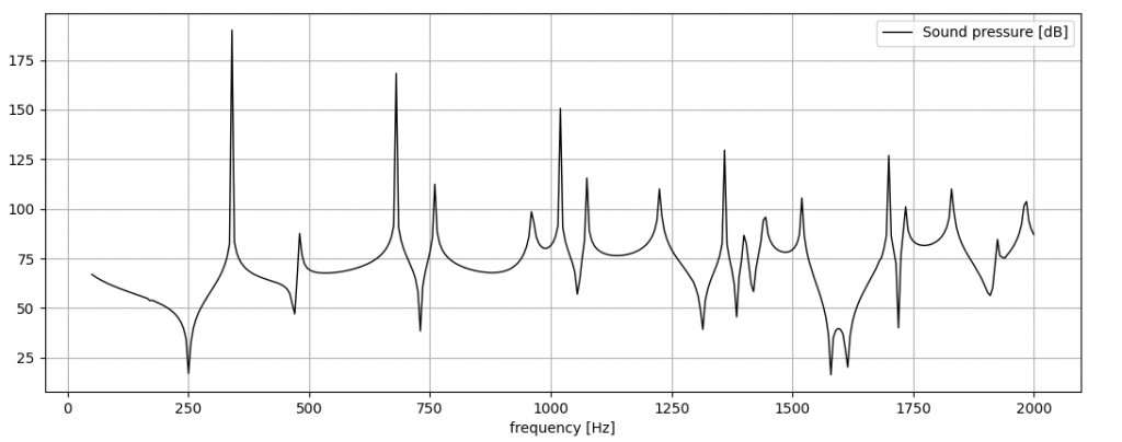
The last time a modal analysis has been performed on a parallepipedic cavity and all the modal shapes have been computed up to the desired frequency. The coincidence between (some) of the eigenfrequencies and the peaks in the sound pressure spectrum has been highlighted.
While modal analysis itself is a good tool to investigate the acoustic behavior of a cavity, its reputation does not come from the fancy animations and from an eigenfrequency list. It represents the foundation of Modal Superposition, that brings full spectral data while saving a huge amount of computation time.
Mathematical derivation
The system of equations that corresponds to a system of equation, derived from the weak form of the Helmholtz equation, is written as follows:
( \bm{K} + j\omega\bm{C} – \omega^{2}\bm{M} )\bm{\hat{p}} =\bm{Q}
Usually the damping matrix \bm{C} is neglected to build the following eigevalue problem:
( \bm{K} – \omega_{m}^{2}\bm{M} )\bm{\Phi_{m}} = 0 with m = 1,2, … , N
Where the martices dimension is n \times n, where n is the number of DOFs of the system.
The mode shapes \bm{\Phi_{m}} can be arranged in a rectangular N\times n matrix \bm\Phi, making the derivation more convenient.
The Modal Superposition technique states that the sound pressure can be written as a linear combination of the acoustic modes:
\bm{\hat{p}} = \sum_{m=1}^{N} \phi_{m} \bm{\Phi_{m}}
Or, in matrix form:
\bm{\hat{p}} = \bm{\Phi \phi}
where \phi_{m} are the modal participation factors, grouped in the vector \bm{\phi}.
By putting the expression above in the initial equation we get:
(\bm{K} + j\omega\bm{C} – \omega^{2}\bm{M} )\bm{\Phi \phi} =\bm{Q}
that is:
\bm{K}\bm{\Phi \phi} + j\omega\bm{C}\bm{\Phi \phi} – \omega^{2}\bm{M} \bm{\Phi \phi} =\bm{Q}
multiplying both sizes by \bm{\Phi}^T the following system is obtained
(\bm{\Phi}^T\bm{K}\bm{\Phi} + j\omega\bm{\Phi}^T\bm{C}\bm{\Phi } – \omega^{2}\bm{\Phi}^T\bm{M} \bm{\Phi}) \bm{\phi} =\bm{\Phi}^T\bm{Q}
where the N\times N matrices
\bm{K}_{a}=\bm{\Phi}^T\bm{K}\bm{\Phi}
\bm{M}_{a}=\bm{\Phi}^T\bm{M}\bm{\Phi}
\bm{C}_{a}=\bm{\Phi}^T\bm{C}\bm{\Phi}
are, respectively, the modal stiffness, modal mass and modal damping matrices. Due to the orthogonality of \bm{\Phi}, it can be shown that the modal stiffness and modal mass matrices \bm{K}_{a}, \bm{M}_{a} are diagonal. The modal damping matrix \bm{C}_{a} is usually written as a combination of the other two, as follows:
\bm{C}_{a} = \alpha\bm{K}_{a}+\beta\bm{M}_{a}
Once the system is set, the unknown modal participation factors can be computed. This operation, compared to the solution of the initial system, is way easier and faster. The first reason is that the matrices are diagonal. Furthermore, if the number of extracted modes N is small enough compared to n, the resulting system is a lot smaller than the initial one, killing the computation time. This is valid for mid-low frequencies, in which the number of modes is small.
Once the modal participation factor vector is computed, the pressure field can be obtained from the relation \bm{\hat{p}} = \bm{\Phi \phi}.
To sum up, there are two computation steps: the first one is the modal extraction (eigenvalue problem), while the second one is the solution of the reduced system. In the right conditions, the sum of these two steps is a lot smaller than the solution of the initial systems, as shown in the following steps:
Case setup
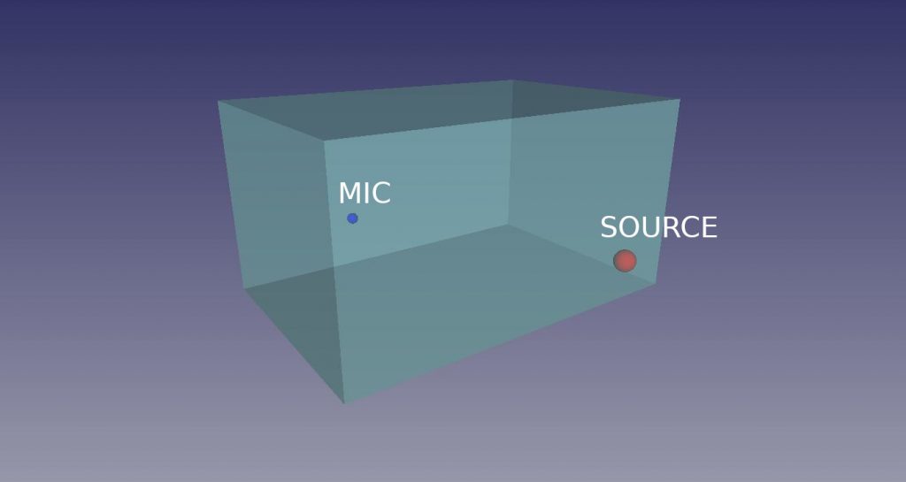
The same case presented before is used for the comparison. This means that geometry, the mesh and the mic and source position remain the same. This is how it looks:
After the extraction of the modes, the \bm{\phi} matrix has been built and exported. This can be easily done thanks to the petsc4py module. Using the same variable names used before, the creation, assembly and export are done as follows:
U = PETSc.Mat().create()
U.setType("dense")
U.setSizes([size_matrices, nconv])
U.setFromOptions()
U.setUp()

for i in range(nconv):
    U.setValues(range(size_matrices), i,  eig_vectors[i])

U.assemble()

viewer_U = PETSc.Viewer().createBinary("U.dat", mode=PETSc.Viewer.Mode.WRITE, comm=MPI.COMM_WORLD)
viewer_U(U)
The number of extracted modes is about 100. The general rule of thumb states that the modes extraction has to reach a factor of 1.5 times the maximum frequency. In my experience, 1.2 or 1.3 can be enough, if the modal density is not too low. Anyway, please, keep in mind that this is depending on the particular system, so. . . Just do your sensitivity analysis! It is always worth it!
We can now import the modes and, afterwards, it is just a matter of matrix multiplications. We discard the damping matrix, since the problem has rigid walls. Next, the modal participation factors have been computed using a KSP Linear Solver from the PETSc library.
Results
The comparison between the sound pressure spectrum at the mic location, computed with the two methods (Direct and Modal) is the following:
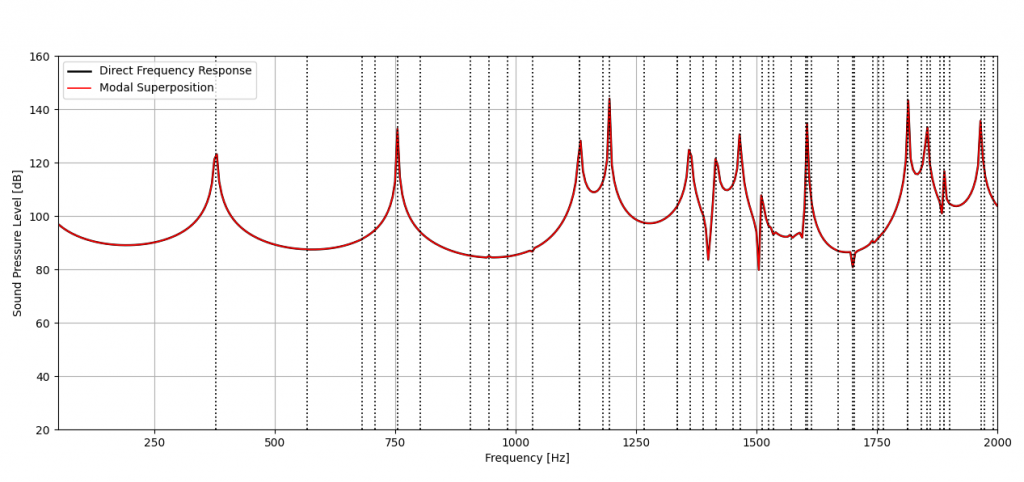
The spectra are identical. What is the gain of such a mathematical complication? Check it out:
Direct Frequency Response computation time: 60 min
Modal Extraction + Superposition computation time: 1 min
The direct method results 60 time slower than the modal method. Keep in mind that such factor grows with the number of DOFs.
Plus, the modal approach gives the contribution of each mode to the sound pressure spectrum:
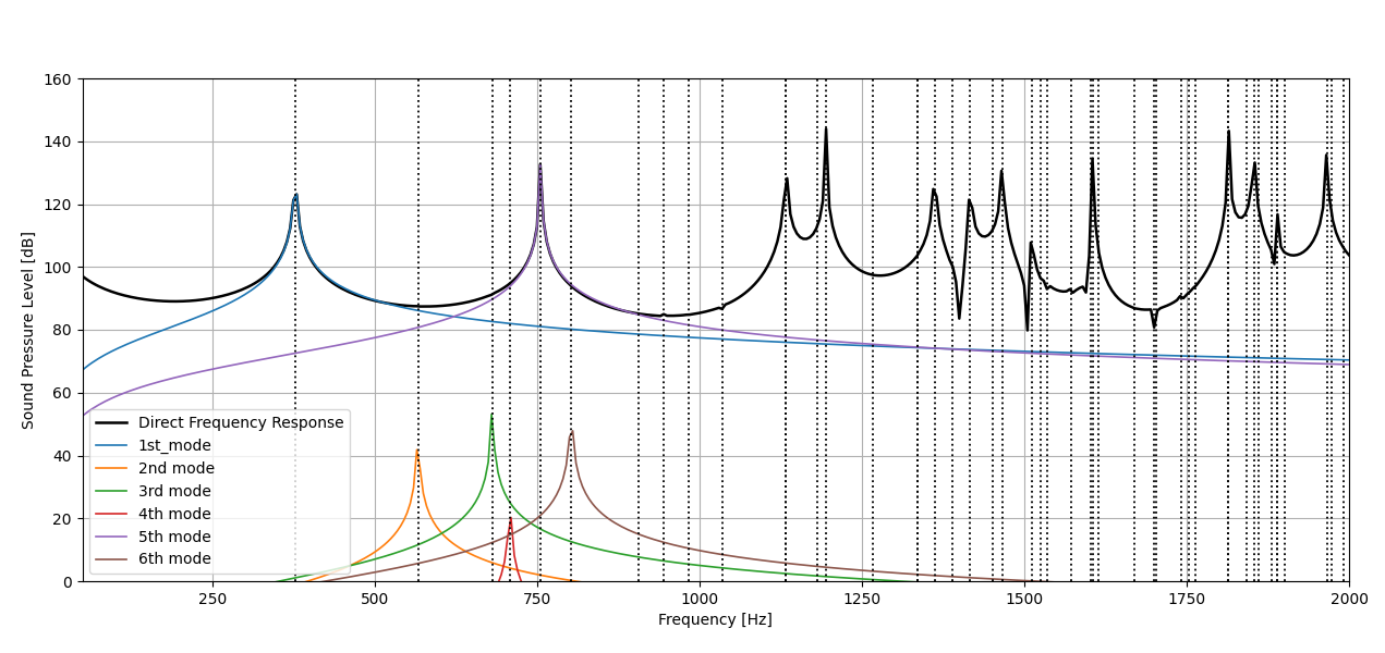
In which you can see that, due to the source/mic position, only the 1st and 5th modes contribute to the spectrum up to about 1000 Hz. The 2nd, 3rd, 4th modes contribution is negligible.
In order to understand the importance of the choice of the number of extracted modes, the spectrum with different values of N is shown:
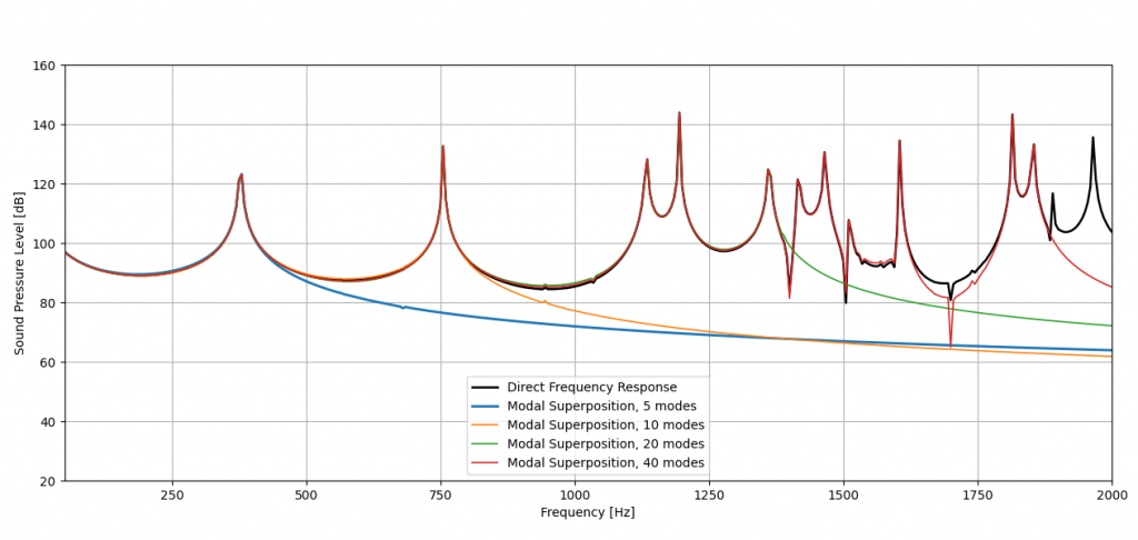
This shows how the accuracy of the method gets better as we increase the number of extracted modes N.
In conclusion, the Modal Superposition approach is very helpful. Taking advantage of the vibrating nature of a system, it projects the solution in the modal space. This, while complicating the mathematical formulation, makes a huge difference in terms of computation time reduction.
Pay attention to the choice of the maximum frequency up to which the modes must be extracted: it is crucial for the accuracy. After that, some important considerations have to be done in case an impedance boundary condition is applied. This will be a good topic for the future. . . Stay tuned!!!