2D Helmholtz equation with FEniCSx: point source in a square room

Introduction

This is the first article of a long series. My goal is to explain the process of performing a full aero-vibro-acoustic simulation on a real system, of industrial interest. This is what I currently do in my daily job, in which I use commercial software (coming from Siemens, ANSYS, MSC).

Since these softwares don’t allow to go deeper into the code and the algorithms used to get to the solution, I decided to use, in most of my examples, an open source software of a special kind: FEniCS. While handling all the matrix assembly, quadrature and actual solving of the final sistem of equation, it allows the user to write a custom differential equation, as long as it is written in its weak form. See here for more details about FEniCS.

If we really want to reach the goal of performing a full aero-vibro-acoustic simulation, we have to start easy. This is the workflow of such a simulation:

Basically, we derive the acoustic source field from a CFD simulation, then we make it propagate inside a coupled vibro-acoustic FEM.

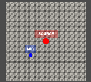
Right now, we are going to start from the acoustic side. How simple we can get in order to learn how to perform a simulation with FEniCS? Let’s build a 2D square room with rigid walls and let’s put a point source (monopole) in its center.

The Helmholtz equation in weak form

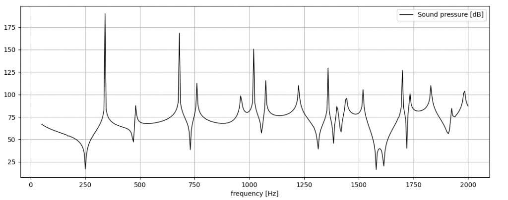
Our goal is to derive the sound pressure spectrum within a given range of frequency, in a specified point and plot the sound pressure field in the entire domain at given frequencies.

In order to get this, we need to solve numerically the inhomogeneous form of the Helmholtz equation, which, in cartesian coordinates, is expressed like this:

$\nabla^{2}\tilde{p}+k^{2}\tilde{p}=-j\omega\rho_{0}\tilde{q}_{m}$

in which $\tilde{p}$ is the complex sound pressure, $k$ is the acoustic wavenumber, $\omega$ is the angular frequency, $\rho_{0}$ the the average density of the fluid and $\tilde{q}_{m}$ the specific volume velocity, that can be written as follows:

$\tilde{q}_{m}=Q\delta(\textbf{x}-\textbf{x}_{0})$

where $Q$ is the source volume velocity and $\delta(\textbf{x}-\textbf{x}_{0})$ is the Dirac delta applied on the point $\textbf{x}_{0}$ .

The weak form of the Helmholtz equation, using the same notation above, is the following:

$\int_{\Omega} \nabla w \cdot \nabla p d\Omega + \int_{\Omega}k^{2}wp d\Omega = -\int_{\Omega}j\omega\rho_{0} w Q\delta(\textbf{x}-\textbf{x}_{0}) d\Omega$

In which $w$ represents the test function.

You can notice that we are not considering any boundary condition. We can ignore them for now, since the abscence of the BC term in the weak formulation automatically implies a zero flux BC that, in acoustics, means rigid walls. Soon we will explain in details the different BCs and their physical meaning in acoustics.

If you want more details on how to get the weak form from the original equation, you can see the following links:

https://www.comsol.it/multiphysics/finite-element-method

https://jorgensd.github.io/dolfinx-tutorial/chapter1/fundamentals.html

Coming, respectively, from COMSOL and FEniCS documentation.

FEniCS

Now let’s get to FEniCS. In order to use it with proficiency, you need to have a basic knowledge of python programming language. On youtube you can find tons of courses about python that start from “hello world” and get to AI programming. It’s on you which one to choose, depending on your needs.

Before we start coding, my advise is to check out the FEniCS tutorial by J. S. Dokken, that explains how the FEniCS modules (UFL,DOLFINx,BASIx, etc.) work togheter. This is the link:

https://jorgensd.github.io/dolfinx-tutorial/index.html

Finally, if you want to implement your version of the code or extend the following code and you need help on it, subrscribe to the FEniCS forum and post your question. The answers come from the staff almost instantly, it’s incredible! Here you find the forum:

https://fenicsproject.discourse.group/

Start the script with the import of the necessary modules:

import numpy as np
import ufl
from dolfinx import geometry
from dolfinx.fem import Function, FunctionSpace, assemble_scalar, form, Constant
from dolfinx.fem.petsc import LinearProblem
from dolfinx.io import XDMFFile
from dolfinx.mesh import create_unit_square
from ufl import dx, grad, inner
from mpi4py import MPI
from petsc4py import PETSc

The mesh will be generated through a DOLFINx module, since we are handling with a simple geometry, but later on we will create it in gmsh and import it in FEniCS. We need to define the polynomial degree of the elements, the number of elements for each direction of the mesh:

# approximation space polynomial degree
deg = 2

# number of elements in each direction of msh
n_elem = 64

msh = create_unit_square(MPI.COMM_SELF, n_elem, n_elem)
n = ufl.FacetNormal(msh)

Then we define the frequency range and the mic position:

#frequency range definition
f_axis = np.arange(50, 2005, 5)

#Mic position definition
mic = np.array([0.3, 0.3, 0])

Now we get to the FEniCS problem build. First of all, a function space V is created on the mesh, defining the type of element we choose (“CG” means Lagrange elements). This operation will select the basis functions necessary for the finite element formulation. Then, we define some empty function, based on the function space V, that will be the trial, test and load functions (u, v, f).

# Test and trial function space
V = FunctionSpace(msh, ("CG", deg))
u = ufl.TrialFunction(V)
v = ufl.TestFunction(V)
f = Function(V)

Next step is the definition of the monopole source. Since the Dirac delta implementation is not yet available on DOLFINx, we need to define it through the limit of a normal distribution as the variance becomes small. I will update the code once the Dirac delta will be implemented.

# Source amplitude
Q = 0.0001

#Source definition position = (Sx,Sy)
Sx = 0.5
Sy = 0.5

#Narrow normalized gauss distribution
alfa = 0.015
delta_tmp = Function(V)
delta_tmp.interpolate(lambda x : 1/(np.abs(alfa)*np.sqrt(np.pi))*np.exp(-(((x[0]-Sx)**2+(x[1]-Sy)**2)/(alfa**2))))
int_delta_tmp = assemble_scalar(form(delta_tmp*dx)) #form() l'ho scoperto per sbaglio. Senza esplode.
delta = delta_tmp/int_delta_tmp

Like in every FE analysis, we define material properties (air):

# fluid definition
c0 = 340
rho_0 = 1.225
omega = Constant(msh, PETSc.ScalarType(1))
k0 = Constant(msh, PETSc.ScalarType(1))

Finally, we define the load f and the two sides of the equation, written in the UFL language that resembles the weak form of the equation itself, a (LHS) and L (RHS):

#building the weak form
f = 1j*rho_0*omega*Q*delta
a = inner(grad(u), grad(v)) * dx - k0**2 * inner(u, v) * dx
L = inner(f, v) * dx

We can now build the proglem through the command LinearProblem(), after defining the wanted variable uh:

#building the problem
uh = Function(V)
uh.name = "u"
problem = LinearProblem(a, L, u=uh, petsc_options={"ksp_type": "preonly", "pc_type": "lu"})

The following code is the core of the problem. After the initialization of the p_mic array, which will contain the sound pressure at the mic point for every frequency, we update the values for the wavenumber and then we solve the problem through the command problem.solve():

p_mic = np.zeros((len(f_axis),1),dtype=complex)
# frequency for loop
print(" ")
for nf in range(0,len(f_axis)):
    print ("\033[A                             \033[A")
    freq = f_axis[nf]
    print("Computing frequency: " + str(freq) + " Hz...")  



    # Compute solution
    omega.value =f_axis[nf]*2*np.pi
    k0.value = 2*np.pi*f_axis[nf]/c0
    problem.solve()

Inside the for loop this code is needed to compute the sound pressure at the desire location and to build the sound pressure array:

    #Microphone pressure at specified point evaluation
    points = np.zeros((3,1))
    points[0][0] = mic[0]
    points[1][0] = mic[1]
    points[2][0] = mic[2]
    bb_tree = geometry.BoundingBoxTree(msh, msh.topology.dim)
    cells = []
    points_on_proc = []
    # Find cells whose bounding-box collide with the the points
    cell_candidates = geometry.compute_collisions(bb_tree, points.T)
    # Choose one of the cells that contains the point
    colliding_cells = geometry.compute_colliding_cells(msh, cell_candidates, points.T)
    for i, point in enumerate(points.T):
        if len(colliding_cells.links(i))>0:
            points_on_proc.append(point)
            cells.append(colliding_cells.links(i)[0])
    points_on_proc = np.array(points_on_proc, dtype=np.float64)
    u_values = uh.eval(points_on_proc, cells)
    
    #building of sound pressure vector
    p_mic[nf] = u_values
    
print ("\033[A                             \033[A")
print("JOB COMPLETED")

After the computation the data is saved in a .csv file, in the format [frequency, Re(p), Im(p)]

#creation of file [frequency Re(p) Im(p)]
Re_p = np.real(p_mic)
Im_p = np.imag(p_mic)
arr  = np.column_stack((f_axis,Re_p,Im_p))
print("Saving data to .csv file...")
np.savetxt("p_mic_2nd.csv", arr, delimiter=",")

And finally we plot the computed sound pressure level:

#spectrum plot
import matplotlib.pyplot as plt
fig = plt.figure()
plt.plot(f_axis, 20*np.log10(np.abs(p_mic)/2e-5), "k", linewidth=1, label="Sound pressure [dB]")
plt.grid(True)
plt.xlabel("frequency [Hz]")
plt.legend()
plt.show()

This is the output of the code: