Hello everyone! In the last articles the way a FEniCSx code has to be written in order to perform an acoustic simulation has been explored. The 2D case was intended to be simple while keeping the simulation set up as close to a real case as possible.
From now the focus will be on acoustic simulation and acoustics in general. I will still share with you the code, but I will explain only the crucial parts that really make the difference (compared to the previous cases). If you have any questions do not hesitate to contact me here.
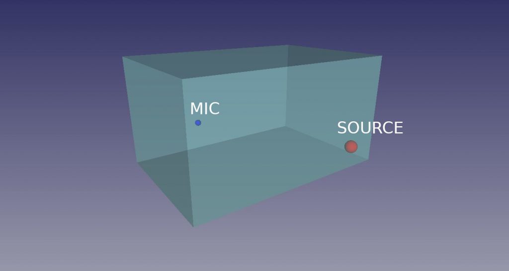
This time a parallelepipedic cavity, which dimensions are 1.5 x 1 x 0.8 m, will be considered. A monopole source, located at the position [0.4, -0.3, 0.1] m, will be the load and a microphone at [0, 0, 1.2] m will be the receiver. The boundary conditions will be rigid walls in the first case while, in the second case, a given impedance will be applied on one of the walls. In order to compute the impedance, a Delany-Bazley-Miki model for a 50 mm layer of porous material (which resistivity was set to 5000) will be used.
The resulting system looks like this:
Geometry and Mesh
After the first two articles, I wanted to follow the workflow that an engineer would actually experience to perform such an analysis. I aim to use only open source software, starting from scratch and getting full acoustic data.
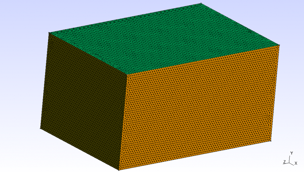
The geometry has been created in FreeCAD (the picture in the previous section is just a screenshot from the software). Then, it has been exported in STEP format. Gmsh was chosen as mesher, since its python API is compatible with FEniCSx. The geometry was easily imported, then the physical groups corresponding to each face and the single volume were defined. The mesh size is set equal to \lambda_{min}/10, that is the minimum wavelength divided by 10, which is a good rule of thumb that ensures a good approximation for the pressure field up to the selected maximum frequency (in our case, 2000 Hz). The resulting mesh size is approximately 17mm, as you can see:
The mesh has been exported in .msh format, that is easily handled by FEniCSx. With a bunch of commands, importing both the mesh and the physical groups will be straightforward.:
The facet_tags variable will be ignored for now, since any explicit boundary condition will be applied in the first case (being them rigid). Anyway, this row will be useful later. The rest of the code is basically the same as the previous cases. FEniCSx recognizes a 3D mesh and sets all the function spaces accordingly. The only thing that has to be added is the third component of the source position:
Sx = 0.4
Sy = -0.3
Sz = 0.1
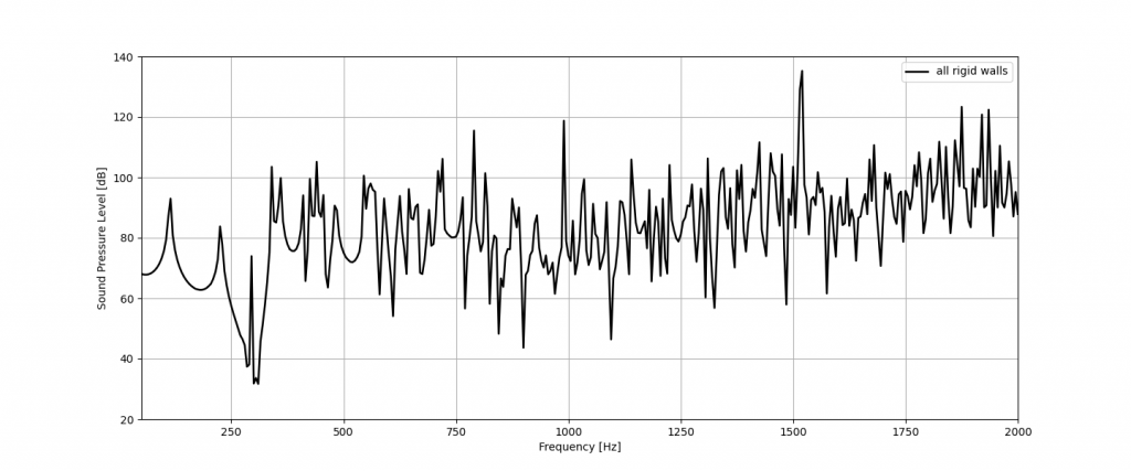
After running the simulation, we can see the sound pressure spectrum in the specified mic location:
All the peaks in the spectrum above represent the cavity modes, where the sound pressure level reaches its highest values. The exported sound pressure fields have been processed in paraview, that is the best suited when plotting 3D complex field. The sound field at some of the analyzed frequencies is shown:
100 Hz
200 Hz
300 Hz
1000 Hz
These pictures show that, when the walls are rigid, the wave is completely stationary. This means that the sound field shape is a superposition of the modes shape for every frequency. More on acoustic modal analysis will be explained later on.
We can now compute the same result in the second case. Some lines need to be added, that are the import and definition of impedance. First we have to initialize the impedance variable
Z_s = Constant(msh, PETSc.ScalarType(1))
Then, the impedance spectrum has to be imported and the complex function has to be defined:
I = np.loadtxt('impedance.csv', delimiter = ",")
Re_Z = I[:,1]
Im_Z = I[:,2]
Z    = Re_Z + 1j*Im_Z
The next step is to define the integration measure ds, needed for the surface integrals definition.
Now it is possible to build the weak form and the solver:
#weak form
f = 1j*rho_0*omega*Q*delta
g = 1j*rho_0*omega/Z_s
a = inner(grad(u), grad(v)) * dx - k0**2 * inner(u, v) * dx +  g * inner(u , v) * ds(5)
L = inner(f, v) * dx

# problem
uh = Function(V)
uh.name = "u"
problem = LinearProblem(a, L, u=uh, petsc_options={"ksp_type": "preonly", "pc_type": "lu"})
Thanks to the facet_tags variable, the impedance boundary condtion ca be applied writing ds(5) in the weak form definition, where 5 is the face ID defined inside gmsh.
This is not the only way but, in my opinion, defining the boundary faces inside gmsh makes the FEniCSx code clearer. Do you agree? Leave your comments below.
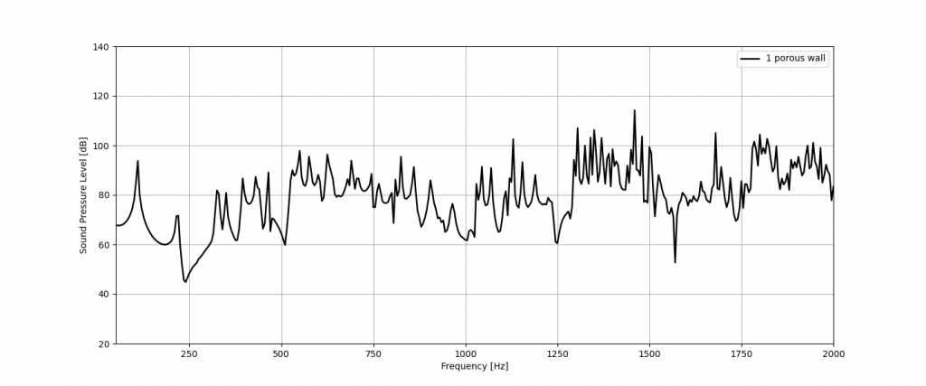
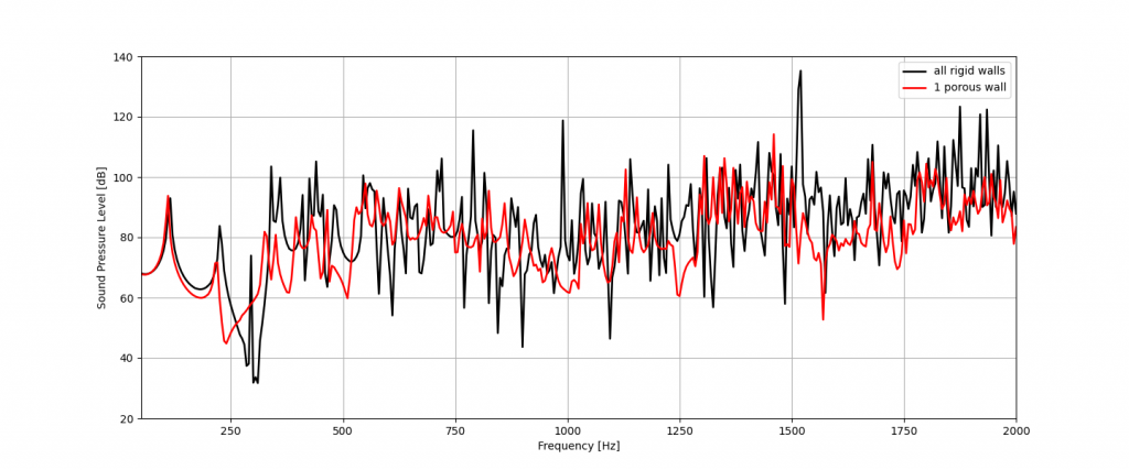
Everything is ready for the computation. After running it, we obtain the results in the same format of the previous case. Here is the sound pressure spectrum:
And finally, you can see the sound pressure fields:
100 Hz
200 Hz
300 Hz
1000 Hz
It is interesting to see the differences in the sound fields between the two cases. At 100 Hz the results are basically equivalent, since the chosen porous layer has no effect at low frequency. At 300 Hz an evident distortion of the field shows up and at 1000 Hz most of the sound pressure is absorbed.
The effect of the porous layer is evident if we overlap the two spectra. In the range close to 1000 Hz the SPL reduction is almost 60 dB.
FEniCSx, in combination with FreeCAD, gmsh and ParaView, shows very good results and optimal usability. If you do not mind spending time scripting and not having a fancy UI, it can do acoustic simulations just like every commercial software.
In next articles, we will explore all the possibilities that such a software can offer to users like us.