Introduction
In previous articles, starting from the Helmholtz equation, the corresponding weak form and the related algebraic system of equation have been shown, then the system has been directly solved. Such an approach is usually called, in commercial softwares, “Direct Frequency Response Analysis” or something similar. If someone of you is familiar with Nastran, it corresponds to SOL 108.
It is well known that, given the nature of waves equation, such a system can be simplified quite a lot (especially at low frequencies) using Modal Analysis. This technique brings to a huge reduction of computation time while preserving the accuracy of the solution (if some important criteria are satisfied).
Before starting, I want to thank Andrea Cicero from AC Acustica for helping me in the setup of the eigensolver.
Mathematical derivation
\int_{\Omega}\nabla w \cdot \nabla p d\Omega – \int_{\Omega}k^{2}wp d\Omega = \int_{\Omega}j\omega\rho_{0} w q d\Omega +\oint_{\partial\Omega}w \frac{\partial p}{\partial n} dS
Corresponds to a system of equation that, in matrix form, looks like below:
( \bm{K} + j\omega\bm{C} – \omega^{2}\bm{M} )\bm{\hat{p}} =\bm{Q}
Where, on the left hand side, \bm{K} is the acoustic stiffness matrix, \bm{C} the acoustic damping matrix and \bm{M} the acoustic mass matrix. On the right hand side, the source vector \bm{Q} takes in account the acoustic load, like a point source.
In order to apply the technique of modal analysis, the undamped acoustic modes have to be computed from the eigenvalue problem associated with the previous equation. Discarding both the damping matrix and the source vector, the generalized eigenvalue problem shows up:
( \bm{K} – \omega_{m}^{2}\bm{M} )\bm{\Phi_{m}} = 0 with m = 1,2, … , N
where the eigenvector \bm{\Phi_{m}} represents a mode shape whose associated eigenvalue is \omega_{m}^{2}, while \omega_{m} is the natural frequency of the mode. N is the number of extracted modes (note that, since the system is continuous, it has an infinite number of modes).
In this article the the natural frequency of the previous system (scaled down, see below) will be computed and their contribution on the sound pressure spectrum coming from a direct frequency analysis will be highlighted.
The next article will focus on the way this set of acoustic modes can be used in a Modal Superposition, which will bring a huge reduction of computation time.
Case setup
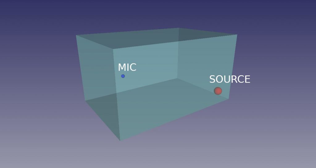
First, the previous simulation has to be modified, in order to avoid high density of modes. The box has been scaled down and its new dimensions are [DIMENSIONI], while the source location and the mic position have been scaled accordingly. It still looks like below:
The mesh dimension did not change, since the maximum frequency of the analysis is still 2000Hz.
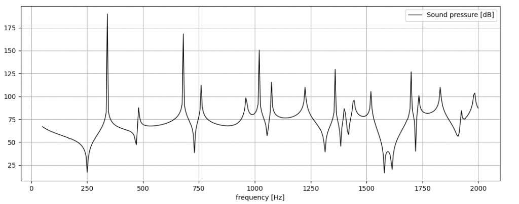
With this setup, the direct computation has been run in the same way, obtaining the following sound pressure spectrum at the mic location:

in which the peaks caused by the acoustic modes are wider and easier to see, compared with the previous case.
Code and SLEPc
from slepc4py import SLEPcThis line has to be added to the previous ones, that remain basically the same.
After importing the mesh (see here), the function space, trial and test function can be created as usual:
# Test and trial function space
V = FunctionSpace(mesh, ("CG", deg))
u = ufl.TrialFunction(V)
v = ufl.TestFunction(V)
In order to solve the eigenvalue problem ( \bm{K} – \omega_{m}^{2}\bm{M} )\bm{\Phi_{m}} = 0 shown before, the acoustic mass and stiffness matrices have to be defined, computed and assembled:
# Stiffness and Mass Matrices
stiff_matrix = inner(grad(u), grad(v)) * dx
mass_matrix  = inner(u, v) * dx

SM = dolfinx.fem.petsc.assemble_matrix(form(stiff_matrix), [])
MM = dolfinx.fem.petsc.assemble_matrix(form(mass_matrix), [])

SM.assemble()
MM.assemble()
Finally, the SLEPc solver can be created and set up. There are al lot of parameters that can be specified but, this time, the EPS solver with GHEP (Generalized Hermitian eigenproblem) problem type will be chosen and a number of 40 modes will be exstracted. The spectral transformation has also to be set up:
# Setup the eigensolver
problem = SLEPc.EPS().create()
A = [ ]
A.append(SM)
A.append(MM)

problem.setDimensions(40)
problem.setProblemType(SLEPc.EPS.ProblemType.GHEP)
problem.setInterval(10,18)
problem.setOperators(SM,MM)

# Setup Spectral Transformation
st = SLEPc.ST().create()
st.setType(SLEPc.ST.Type.SINVERT)
st.setShift(0.1)
st.setFromOptions()

problem.setST(st)

# Solve the eigenproblem
problem.solve()
Once the problem has been solved, the eigenvectors and eigenfrequencies can be extracted:
# Getting the result vectors
xr, xi = SM.createVecs()
nconv = problem.getConverged()
if nconv > 0:
eig_values = []
eig_vectors = []
eig_freq = []
for i in range(nconv):
k = problem.getEigenpair(i, xr, xi)
fn = np.sqrt(k.real)/(2*np.pi)*340
eig_values.append(k)
eig_freq.append(fn)
eig_vectors.append(vect.copy())The eigenvector are shown at the corresponding eigenfrequency. Since their combination rules the sound pressure field, they are better known as “mode shapes”. Here are some of them:


With such a simple geometry, the mode shapes are symmetrical, allowing to compute them analytically. With more complicated shapes, FEM modal analysis is the only way to have the same results.
Lastly, the entire set of eigenfrequency has been plotted below, together with the previous spectrum:

Here you can see that all the peaks correspond to an eigenfrequency, but not every eigenfrequency gives a peak in the spectrum. This strictly depends on the source and mic position. If the source is located in a nodal plane (where the modal amplitude is equal to zero), it will not activate it. The same happens if the microphone is located in such a plane: it will not catch the sound pressure peak.
The next article will show how to use such data to perform a Modal Superposition, that will result in the same spectrum computed.