Introduction
Last time, we introduced the fundamentals of vibroacoustics, providing a detailed explanation of fluid-structure interaction (FSI). We demonstrated how the final system is represented as a combination of individual subsystem matrices, augmented by various coupling terms. A significant challenge arises when the size of such a system expands, leading to excessively high computational times or overwhelming the available computational resources.
To address this issue, we are going to apply the modal approach on the structural part to reduce the computational complexity. The modal approach involves decomposing the system into a set of eigenmodes, as we already explainded here.
System reduction
The system equation for the monolithic approach used in the last article are the folllowing:
\left(\begin{bmatrix} \bf{K_s} & \bf{C_{sa}} \\0 & \bf{K_a} \end{bmatrix} – \omega^2\begin{bmatrix} \bf{M_s} & 0 \\ -\bf{C_{as}} & \bf{M_a} \end{bmatrix}\right) \begin{bmatrix} \bf{\hat{u}} \\ \bf{\hat{p}} \end{bmatrix} = \begin{bmatrix} \bf{0} \\ \bf{F_a}\end{bmatrix}.
While the direct solution of such system (using, as an example a LU decomposition on the entire matrix) gives us the exact solution, we can split the problem in two steps.
1. (Structural) modal extraction
Firstly, we begin by utilizing the principle that the structural displacement can be expressed as a modal superposition, where each natural mode is multiplied by its corresponding modal participation factors:
\bf{\hat{u}} = \bf{\Phi}\phi
As we already know, such modes can be extracted from the following eigenvalue problem:
\left(\bf{K_s} – \omega_m^2 \bf{M_s}\right) \bf{\Phi_m} = 0
where \bf{K_s} and \bf{M_s} are the structural stiffness and mass matrices, while \bf{\Phi_m} is the mode shape vector, that will be the column vector of the mode shapes matrix \bf{\Phi} .
If we substitute \bf{\hat{u}} in the first system, we get:
\left(\begin{bmatrix} \bf{K_s \Phi} & \bf{C_{sa}} \\0 & \bf{K_a} \end{bmatrix} – \omega^2\begin{bmatrix} \bf{M_s \Phi} & 0 \\ -\bf{C_{as}\Phi} & \bf{M_a} \end{bmatrix}\right) \begin{bmatrix} \bf{\phi} \\ \bf{\hat{p}} \end{bmatrix} = \begin{bmatrix} \bf{0} \\ \bf{F_a}\end{bmatrix}
Like we did before, we can multiply the right side of the first row by \bf{\Phi^T} to obtain the final system:
\left(\begin{bmatrix} \bf{\Phi^T K_s \Phi} & \bf{\Phi^T C_{sa}} \\0 & \bf{K_a} \end{bmatrix} – \omega^2\begin{bmatrix} \bf{\Phi^T M_s \Phi} & 0 \\ -\bf{C_{as}\Phi} & \bf{M_a} \end{bmatrix}\right) \begin{bmatrix} \bf{\phi} \\ \bf{\hat{p}} \end{bmatrix} = \begin{bmatrix} \bf{0} \\ \bf{F_a}\end{bmatrix}
Solving such system with whatever approach (LU for example) will give us the unknown vector, where we get both the sound pressure field and the modal participation factors field.
Test case: sound transmission through a box
A spherical source is located inside a plastic box (E = 4 GPa, \rho = 1000 kg/m^3), which thickess is equal to 2 mm. The output of the problem will be the sound pressure level at the microphone location, outside of the box. The only way for the sound to get out of the box is through transmission, that is modeled with a strong coupling.

First of all, we solve the eigenvalue problem on the structural domain, getting the mode shapes matrix \Phi. Its columns represent a vector field, which can be plotted for the first modes:


Then we apply the modal superposition method, as previously discussed, to obtain the pressure spectrum at the microphone location. Below, we compare these results with those obtained using the direct approach to solve the same problem.:

While the results are quite satisfactory, it’s important to note that the computation time was significantly reduced, from 16 hours to just 4 hours, and the maximum RAM requirement decreased from 23 GB to 18 GB.
Despite the large number of structural modes in the frequency range (approximately 200), employing modal superposition proved to be greatly beneficial. Should the number of modes within your specific frequency range be fewer, the reduction in both time and hardware requirements could be even more pronounced.
Following, a pretty snapshot of the sound pressure field outside of the box at 200 Hz:

Hello,
hope every thing is greate,
I’m a researcher working in area of FSI of hyperelasric matrial and vibro – aeroacoustic signature. I’m currently studying the effect of aortic valve atenosis on the heart sound and currently using LSdynao to do this job. I used befor the two way coupling to sinulate vavle movement with LES model and then extract the pressure wave and pass it to other acoustic analogies to predict the sound generated.
I see you propose a solid method for Vibro acoustic simulation and was wondering if this cound by any level help in my case?
can I exploite your codes in conjunction with other commercial softwares like ANSYS, or opensource like OpenFOAM.
Thanks in advance