Introduction
Vibroacoustics is an interdisciplinary domain that deals with the interaction between mechanical vibrations and acoustic waves. As computational methods gain importance in predicting and controlling noise and vibration, computational vibroacoustics has become a cornerstone for engineers and researchers. In this article we are going to understand how the coupling between the equations is handled.
Sound and vibration equations
Suppose that we have the following system:

Where an acoustic domain, \Omega_a is coupled with an elastic domain \Omega_s through the surface \partial \Omega_{int}.
We can write the weak form for linear elastodynamics and linear acoustics, resulting in the following system:
Linear Elastodynamics:
\int_{\Omega_s} \sigma(\mathbf{u}) : \epsilon (\mathbf{w}) d\Omega_s – \int_{\Omega_s} \rho_s\omega^2 \mathbf{u\cdot w} d\Omega_s = \int_{\partial\Omega_{int}} -p\mathbf{n_s \cdot w} d\partial\Omega_{int}
Linear Acoustics:
\int_{\Omega_a}\nabla p \cdot \nabla v d \Omega_a – \int_{\Omega_a}k_a^2p v d \Omega_a = \int_{\Omega_a} j\omega\rho_a q v d \Omega_a + \int_{\partial\Omega_{int}} \rho_a \omega^2 \left(\mathbf{u \cdot n_a}\right) v d\partial\Omega_{int}
For the elastodynamics equation, \Omega_s represents the solid domain over which the integral is evaluated. The stress tensor \sigma(\mathbf{u}) and the strain tensor \epsilon(\mathbf{w}) are functions of the displacement field \mathbf{u} and the test function \mathbf{w} , respectively. The term \rho_s denotes the density of the solid, and \omega stands for the angular frequency. On the boundary \partial\Omega_{int} , p represents the acoustic pressure and \mathbf{n_s} is the outward-pointing normal vector to the boundary from the solid side.
Similarly, for the acoustics equation, \Omega_a denotes the acoustic domain. Here, p is the acoustic pressure, and v is the acoustic test function. The wave number k_a and density \rho_a correspond to the acoustic medium. The source term q represents any external acoustic source within the domain. Finally, \mathbf{u \cdot n_a} on the boundary \partial\Omega_{int} represents the projection of the solid’s velocity along the outward-pointing normal vector \mathbf{n_a} from the acoustic side.
With the usual Finite Element Method tecniques, it can be shown that such equations are assembled in the following algebraic systems of equations:
\left(\bf{K_s} – \omega^2 \bf{M_s}\right) \bf{\hat{u}} = -\bf{C_{sa}} \bf{\hat{p}}
\left(\bf{K_a} – \omega^2 \bf{M_a}\right) \bf{\hat{p}} = \bf{F_{a}} \omega^2 \bf{C_{as}}\bf{\hat{u}}
In the given equations, \bf{K_s} and \bf{K_a} are the stiffness matrices for the solid and acoustic domains, respectively. \bf{M_s} and \bf{M_a} represent the elastic and acoustic mass matrices. The vectors \bf{\hat{u}} and \bf{\hat{p}} correspond to the displacement and pressure at the nodes of the solid and acoustic meshes. The matrices \bf{C_{sa}} and \bf{C_{as}} describe the coupling between the solid and the acoustic domains, commonly appearing from the pressure-velocity coupling in the boundary conditions. Finally, \bf{F_a} encapsulates any external forces or acoustic sources within the acoustic domain. These equations represent the assembled forms of the governing equations for vibroacoustics, transformed into the frequency domain and including coupling terms, making them suitable for numerical solutions using methods like the Finite Element Method.
The equation above can be coupled and solved in two different ways:
1. Monolithic Approach:
In the monolithic strategy, the coupled elastodynamics and acoustics equations are assembled into a single, global system expressed as
\left(\begin{bmatrix} \bf{K_s} & \bf{C_{sa}} \\0 & \bf{K_a} \end{bmatrix} – \omega^2\begin{bmatrix} {M_s} & 0 \\ \bf{C_{as}} & \bf{M_a} \end{bmatrix}\right) \begin{bmatrix} \bf{\hat{u}} \\ \bf{\hat{p}} \end{bmatrix} = \begin{bmatrix} \bf{0} \\ \bf{F_a}\end{bmatrix}.
This global system can be solved using direct solvers like LU decomposition.
2. Partitioned Approach:
In this approach, the solid and fluid equations are solved iteratively and sequentially. One might initialize an estimate for \bf{\hat{u}}^{(0)} or \bf{\hat{p}}^{(0)} and proceed as follows:
– Algorithm Example:
1. Solve for \bf{\hat{p}}^{(k)} using \left(\bf{K_a} – \omega^2 \bf{M_a}\right) \bf{\hat{p}}^{(k)} = \bf{F_{a}} + \omega^2\bf{C_{as}}\bf{\hat{u}}^{(k-1)}.
2. Solve for \bf{\hat{u}}^{(k)} using \left(\bf{K_s} – \omega^2 \bf{M_s}\right) \bf{\hat{u}}^{(k)} = -\bf{C_{sa}} \bf{\hat{p}}^{(k)} .
3. Check for convergence; if not met, return to Step 1.
The monolithic approach captures strong couplings effectively but may be computationally expensive, while the partitioned approach offers modularity and computational efficiency at the risk of convergence issues in correspondance of the eigenfrequencies of both systems.
Test case: sound transmission through a square plate
We are going to apply what we have learned to an actual simulation, which will be solved using the monolithic approach.
Suppose we have two fluid domains (air), that interface with a square plate. We will place a monopole source on one side and measure the sound pressure level on the other. The cavities will have rigid walls everywhere except on surface S_{imp}, where the impedance \rho_a c_a will be assigned.
The plate, made of generic plastic (E = 2 GPa, \nu = 0.4 and \rho_s = 1000 kg/m^3 is clamped on all four borders.

In this configuration, the problem is strongly coupled. Both the structure and acoustic modes will determine the spectrum in the downstream microphone, shown below:

This is just one spectrum. We can easily compute the spectrum at any required location. This capability is useful for characterizing the plate’s Transmission Loss and Absorption Coefficient (it’s low, but not zero!). Further simulations can be conducted to enhance the structure’s effect on cavity modes, with the aim of dampening them. Below, we present a (paraview) animation illustrating the formation of the acoustic field at 1000 Hz:
Here, you can observe the plate’s impact on the proximal acoustic field. In contrast, at greater distances, the field is predominantly characterized by longitudinal modes. This simulation allows you to identify the transition region between the plate-influenced and plate-uninfluenced acoustic fields.
How would you use a vibro-acoustic simulation tool? Let me know in the comments below!