Introduction
Locally conformal perfectly matched layers (LC-PML) are an essential technique in computational acoustics and wave propagation simulations in general. They are designed to efficiently absorb outgoing waves and prevent unwanted reflections at the boundaries of computational domains. In this article, we will explore the implementation of LC-PML in FEniCSx, and discuss its advantages and disadvantages.
Simulating wave propagation in unbounded domains poses significant challenges due to the need to truncate the computational domain. LC-PML offers an effective solution by introducing absorbing layers that mimic an infinite domain. The advantages of LC-PML are the same of conventional PML, like improved accuracy, reduced reflections, and the ability to simulate unbounded domains. Furthermore, LC-PML allows to build PML layers on top of arbitrary shaped domains. You don’t have to stick with parallelepipeds and spheres anymore!
In this implementation, the layer will be automatically built by gmsh, once the PML surface are provided.
Theory
This work is based on the following papers:
[1] Y. Mi, X. Yu – Isogeometric locally-conformal perfectly matched layer for time-harmonic acoustics, 2021
[2] H. Beriot, A. Modave – An automatic perfectly matched layer for acoustic finite element simulations in convex domains of general shape, 2020
[3] O. Ozgun, M. Kuzoglus – Locally-Conformal Perfeclty Matched Layer implementation for finite element mesh truncation, 2006
[4] O. Ozgun, M. Kuzoglus – Near-field performance analysis of locally-conformal perfectly matched absorbers via Monte Carlo simulations, 2007
We want to solve the following Helmholtz problem:
\begin{cases} {\nabla^{2}\tilde{p} + k^{2}\tilde{p}=-j\omega\rho_{0}\tilde{q}_{m}}& {\text{on $\Omega$} }\\ {\frac{\partial \tilde{p}}{\partial n}= q }& {\text{on $\partial{\Omega}$} }\\ {\lim_{r \to \infty} r\left( \frac{\partial \tilde{p}}{\partial n} + jk\tilde{p}\right)}&{}\\ \end{cases}
In which the Sommerfeld radiation condition describes the slow decay of the waves at large distance from the source. There is one “tiny” problem: our domain is finite!
To explain how LC-PML works, let’s suppose that we have a physical domain of arbitrary convex shape, surroundend by a conformal PML. Lets define a specific curvilinear coordinate system (\xi_{1}, \xi_{2},\xi_{3}) such that \xi_1 is the distance to the closest point belonging to \Gamma_{i} and \xi_{2},\xi_{3} are provided by a local parametrization of \Gamma_{i} . The local parametrization, as explained in [2], is given by:
\frac{\partial\mathbf{n}}{\partial\xi_{i}} = \kappa_{i} \mathbf{t}_{i} \quad \text{where} \quad \mathbf{t}_{i} = \frac{\partial \mathbf{p}}{\partial \xi_{i}} \quad \text{for} \quad i=2,3

where t_1 and t_2 are the principal curvatures of \Gamma_i.
The curvilinear transformation that brings from such system back to the cartesian coordinate system is:
\mathbf{x}(\xi_{1},\xi_{2},\xi_{3}) = \mathbf{p}(\xi_{1},\xi_{2}) + \xi_{1} \mathbf{n} (\xi_{1},\xi_{2})
Since we need it later, we calculate the Jacobian matrix of this transformation:
\mathbf{J}_{x/\xi} = \frac{\partial ( x, y,z)}{\partial \left( \xi_{1},\xi_{2},\xi_{3} \right)} = \left[ \frac{\partial \mathbf{x}}{\partial \xi_{1}} \quad \frac{\partial \mathbf{x}}{\partial \xi_{2}} \quad \frac{\partial \mathbf{x}}{\partial \xi_{3}} \right] = \left[ \mathbf{n} \quad (1+\kappa_{2} \xi_{1} ) \mathbf{t_{2}} \quad (1+\kappa_{3}\xi_{1})\mathbf{t_{3}} \right] = \left[ \mathbf{n} \quad h_{2}\mathbf{t_{2}} \quad h_{3}\mathbf{t_{3}} \right] \quad \text{(1)}
The core of Locally-Conformal PML approach is that the complex coordinate stretch (that is, the conventional transformation that makes the PML absorb all the incoming waves) is applied only on the normal direction \xi_1:
\tilde{\xi}_{1} (\xi_{1}) = \xi_{1} + \frac{1}{jk}f(\xi_{1}) \quad \text{(2)}
For which the Jacobian matrix is:
\mathbf{J}_{\tilde{\xi}/\xi} = \frac{\partial ( \tilde{\xi_{1}},\tilde{\xi_{2}},\tilde{\xi_{3}})}{\partial \left( \xi_{1},\xi_{2},\xi_{3} \right)} = \begin{bmatrix} {\frac{d \tilde{\xi}_{1}}{d\xi_{1}}}& {0 }& {0 }\\ {0 }& {1 }& {0 }\\ {0 }& {0 }& {1 }\\ \end{bmatrix} = \begin{bmatrix} {1+ \frac{1}{jk}\sigma }& {0 }& {0 }\\ {0 }& {1 }& {0 }\\ {0 }& {0 }& {1 }\\ \end{bmatrix}= \begin{bmatrix} {s_{1} }& {0 }& {0 }\\ {0 }& {1 }& {0 }\\ {0 }& {0 }& {1 }\\ \end{bmatrix}
With this in mind, we can compute the total jacobian J_{PML}, that brings us from the complexified cartesian coordinates to the real cartesian coordinates.
Thanks to the chain rule, we can split it as follows:
\mathbf{J}_{PML} = \frac{\partial \left( \tilde{x},\tilde{y},\tilde{z} \right)}{\partial \left( x,y,z \right)}=\frac{\partial \left( \tilde{x},\tilde{y},\tilde{z} \right)}{\partial (\tilde{\xi}_{1},\tilde{\xi}_{2},\tilde{\xi}_{3} )} \frac{\partial ( \tilde{\xi}_{1},\tilde{\xi}_{2},\tilde{\xi}_{3} )}{\partial \left( \xi_{1},\xi_{2},\xi_{3} \right)} \frac{\partial \left( \xi_{1},\xi_{2},\xi_{3} \right)}{\partial \left( x,y,z \right)}
Where the steps represent:
- the transformation from Cartesian coordinates to curvilinear coordinates in the complex space
- the use of the complex stretch to come back in the real space
- the transformation from curvilinear coordinates to Cartesian coordinates in the real space
The first jacobian matrix can be computed from the previous formula, with the difference of complex \xi_1:
\mathbf{J}_{\tilde{x}/\tilde{\xi} } = \frac{\partial ( \tilde{x}, \tilde{y},\tilde{z} )}{\partial \left( \tilde{\xi}_{1},\tilde{\xi}_{2},\tilde{\xi}_{3} \right)} = \left[ \mathbf{n} \quad (1+\kappa_{2} \tilde{\xi}_{1} ) \mathbf{t_{2}} \quad (1+\kappa_{3} \tilde{\xi}_{1})\mathbf{t_{3}} \right] = \left[ \mathbf{n} \quad (1+\kappa_{2} \tilde{\xi}_{1} ) \mathbf{t_{2}} \quad (1+\kappa_{3} \tilde{\xi}_{1})\mathbf{t_{3}} \right] = \left[ \mathbf{n} \quad s_{2} h_{2}\mathbf{t_{2}} \quad s_{3} h_{3}\mathbf{t_{3}} \right]
\text{where} \quad s_{i} = 1-\frac{\kappa_{i}}{jkh_{i}}f(\xi_{1})
Since the second jacobian has been computed already, we are only missing the last one. Notice that is just the inverse of (1):
\mathbf{J}_{\xi/x} = \frac{\partial ( \xi_{1},\xi_{2},\xi_{3})}{\partial \left( x, y,z \right)} = \left[ \mathbf{n} \quad h_{2}^{-1}\mathbf{t_{2}} \quad h_{3}^{-1}\mathbf{t_{3}} \right]
We can now compute the PML Jacobian matrix:
\mathbf{J}_{PML} = \frac{\partial \left( \tilde{x},\tilde{y},\tilde{z} \right)}{\partial \left( x,y,z \right)}=\mathbf{J}_{\tilde{x}/\tilde{\xi} } \mathbf{J}_{\tilde{\xi}/ \xi}\mathbf{J}_{\xi/x}=
= \left[ \mathbf{n} \quad s_{2} h_{2}\mathbf{t_{2}} \quad s_{3} h_{3}\mathbf{t_{3}} \right] \begin{bmatrix} {s_{1} }& {0 }& {0 }\\ {0 }& {1 }& {0 }\\ {0 }& {0 }& {1 }\\ \end{bmatrix} \left[ \mathbf{n} \quad h_{2}^{-1}\mathbf{t_{2}} \quad h_{3}^{-1}\mathbf{t_{3}} \right]= s_{1} \mathbf{n} \mathbf{n^{T}} +s_{2} \mathbf{t_{2}} \mathbf{t_{2}^{T}} + s_{3}\mathbf{t_{3}} \mathbf{t_{3}^{T}}
and its inverse, that is:
\mathbf{J}_{PML}^{-1} = s_{1}^{-1} \mathbf{n} \mathbf{n^{T}} +s_{2}^{-1} \mathbf{t_{2}} \mathbf{t_{2}^{T}} + s_{3}^{-1}\mathbf{t_{3}} \mathbf{t_{3}^{T}}
It is possible to demonstrate that the physics inside the PML is described by an anisotropic version of the Helmholtz equation:
\nabla \cdot \left( \mathbf{\Lambda}_{PML}\nabla \tilde{p} \right)+ \alpha_{PML}k^{2}\tilde{p} = -j\omega\rho_{0} \tilde{q}_{m}
where
\mathbf{\Lambda}_{PML} = \mathbf{J}_{PML}^{-1}\mathbf{J}_{PML}^{-T} det(\mathbf{J}_{PML})=\frac{s_{2} s_{3}}{s_{1}}\mathbf{n} \mathbf{n^{T}} +\frac{s_{1} s_{3}}{s_{2}}\mathbf{t_{2}} \mathbf{t_{2}^{T}} + \frac{s_{1} s_{2}}{s_{3}}\mathbf{t_{3}} \mathbf{t_{3}^{T}}
and
\alpha_{PML} = det(\mathbf{J}_{PML})\,=\,s_{1}s_{2}s_{3}
Implementation
The implementation has been possible thanks to the software gmsh and its powerful python API. The entire code is available on github. If you want to contribute, use it or improve it, click here.
Here we are going to show only the main parts of the code. First, we show how, with the gmsh API, it is possible to extrude the Perfecly Matched Layer, retrieve the principal curvatures, the principal direction and the normal of a given surface:
gmsh.option.setNumber('Geometry.ExtrudeReturnLateralEntities', 0)
e = gmsh.model.geo.extrudeBoundaryLayer(PML_interface_entities, [Num_layers], [d_pml], False)
for sub_surf in bottom_surf:
tags, coord, param = gmsh.model.mesh.getNodes(2, sub_surf, True)
k_2, k_3, t_2, t_3 = gmsh.model.getPrincipalCurvatures(sub_surf,param)
n_1 = gmsh.model.getNormal(sub_surf,param)After this (and after a lot of nodetags sorting and duplicates fixing) the computed variables are projected in the PML cells with the criterion of the minimum distance from the PML interface:
for n in range(len(tags3_nodup)):
            if n in tags3_PML:
                    d_square    = np.sqrt((xx[n] - XX)**2 + (yy[n] - YY)**2 + (zz[n] - ZZ)**2)
                    min_d       = np.min(d_square)
                    min_idx     = np.argmin(d_square)

                    k2_PML[n]   = K22_NODUP[min_idx]
                    k3_PML[n]   = K33_NODUP[min_idx]

                    d[n]        = min_d

                    t2_x_PML[n] = T22_x[min_idx]
                    t2_y_PML[n] = T22_y[min_idx]
                    t2_z_PML[n] = T22_z[min_idx]

                    t3_x_PML[n] = T33_x[min_idx]
                    t3_y_PML[n] = T33_y[min_idx]
                    t3_z_PML[n] = T33_z[min_idx]

                    n_x_PML[n]  = N_x[min_idx]
                    n_y_PML[n]  = N_y[min_idx]
                    n_z_PML[n]  = N_z[min_idx]
In the end, we can create the FEniCSx functions, and write the expressions for scale factors, stretching functions, \Lambda_{PML} and \alpha_{PML}:
# scale factors
h2    = 1 + k2*csi
h3    = 1 + k3*csi

# stretching functions
s1    = 1 + 1/(1j*k0)*sigma
s2    = 1 + k2 * f_csi/(1j*k0*h2)
s3    = 1 + k3 * f_csi/(1j*k0*h3)

# diadic tensors (outer product of the principal directions)
nnT   = as_matrix(np.outer(n,n))
t2t2T = as_matrix(np.outer(t2,t2))
t3t3T = as_matrix(np.outer(t3,t3))

# determinant of J_PML
alpha_PML  = s1*s2*s3

# PML tensor
LAMBDA_PML = s2*s3/s1 * nnT + s1*s3/s2 * t2t2T + s1*s2/s3 * t3t3T
It is now possible to build the weak form in FEniCSx that will solve the problem:
# weak form definition:
f  = 1j*rho_0*omega*Q*delta

a  = inner(grad(u), grad(v)) * dx(1) - k0**2 * inner(u, v) * dx(1)  \
        + inner(LAMBDA_PML*grad(u), grad(v)) * dx(2) - alpha_PML * k0**2 * inner(u, v) * dx(2)

L  = inner(f, v) * dx(1)
Validation
The model has been validated with a monopole source propagating in free field. For such a case, the analytical solution for the pressure is:
p(r) = j \omega \rho_0 Q \frac{e^{-jkr}}{4\pi r}
where Q represents the acoustic volume velocity and r is the distance between the source and the virtual microphone.
Below, the domain used for the comparison:

The automatically generated mesh and the extruded Perfectly Matched Layer is shown:

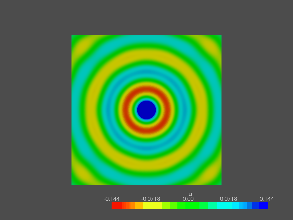
The solver automatically produces two solution fields: the first one contains the PML cells, while in the second one they are removed. It looks like this:

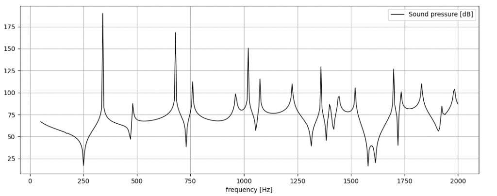
From the user perspective, in this way, the PML “feels” just like another bundary condition. The pressure spectrum is compared (for 1st and 2nd order tetra) with the analytical solution:


Below, the difference between the computed spectra and the analytical one is shown: note that, above 200 Hz the error stays below 0.5 dB:

In the end, the reader has to remember that, even if the code and the model has been calibrated and optimized by the author, there are still some “knobs” that can be customized and are very important for the accuracy of the simulations:
- Number of layers: higher number means better accuracy, but also bigger number of cells and then higher computation time
- Order of the elements: the absorption function \sigma (\xi_1) is usually polynomial or hyperbolic. Higher order element means better representation of the (fast) decay occurring in the layer.
- Total thickness of the layer: at low frequencies the wave needs more physical space to actually decay and make the reflections neglectable. Of course, this increases the total number of elements and then the computation time, again.
Please, take a look at the code, play with it if you want and report any bugs that you can find! Any suggestion that improves the code is also accepted. Have fun!
The code: github.com/bayswiss/autogen_LC_PML
Hi, very nice entry. (I will try to implement it myself)
You have a typo in the coordinate transform from real curvilinear coordinates to real cartesian coordinates,
chi_1 and chi_2 inside the vectors p and n should be chi_2 and chi_3